BLOG

We have a new open-access study out in the current volume of Journal of Geophysical Research that brings together both radar and laser altimetry measurements to assess the mass balance of the Greenland Ice Sheet between 2011 and 2020. Our assessment shows that the ice sheet lost approximately 498 Gt of ice volume, corresponding to approximately 7 mm of global sea-level equivalent during this time. The peak loss year was from April 2019 to April 2020, when the ice sheet lost 1.4 mm of global sea-level equivalent, which is equivalent to losing 15,850 tonnes of ice per second for an entire year. These values reflect only the ice sheet proper, and ignore Greenland’s peripheral glaciers. 

Over the study period, we estimate that approximately 43% of the ice loss was due to ice dynamics (i.e. more iceberg calving). Surface mass balance, or meltwater runoff, was responsible for the remaining approximately 57% of mass loss. This partition of mass loss varies tremendously between ice-sheet catchments and through time. This allows us to see the ice-sheet responding to recent climate forcing at the scale of individual seasons and catchments. Our assessment even resolves mass loss changes at the level of individual glaciers. For example, we can see that after a brief period of ice thickening during 2018 and 2019, Jakobhavn Isbræ has now returned to substantial ice thinning. 

If you’re really into satellite altimetry, we also make a rather unique cross-comparison between ICESat-2 laser measurements and CryoSat-2 radar measurements. While laser altimetry enjoys a near-complete surface scattering of the incoming laser pulse, radar altimetry has substantial volume scattering, meaning that the incoming radar pulse penetrates some depth into the ice sheet. This makes it difficult to assimilate both laser and radar altimetry measurements into a common processing pipeline. But, after applying the necessary volume-scattering correction to the radar measurements, we can assimilate both the ICESat-2 and CryoSat-2 observations into a common framework that shows good agreement (±8 cm/yr) during the common 2019/20 year.

Finally, to be consistent with an open science mandate and help the community move forward as fast as possible, we make the annual (April to April) ice-sheet maps of volume change that we assess at 1 km spatial resolution available for download at: https://datadryad.org/stash/share/gRoJh1JfpF4EA1d_Prsa_KIju9z2hJXWvXE5J1X2d8I. We hope these data will be useful for not only inter-study altimetry comparisons, but also for initializing models that calculate the elastic uplift of Greenland’s bedrock and evaluating ice flow models that simulate recent ice-sheet mass loss. 

Khan, S. A., Bamber, J. L., Rignot, E., Helm, V., Aschwanden, A., Holland, D. M., van den Broeke, M., King, M., Noël, B., Truffer, M., Humbert, A., Colgan, W., Vijay, S., and Kuipers Munneke, P. (2022). Greenland mass trends from airborne and satellite altimetry during 2011–2020. Journal of Geophysical Research: Earth Surface. 127. e2021JF006505. https://doi.org/10.1029/2021JF00650

We have a new open-access study about Greenland Ice Sheet mass balance – or health – in the current issue of Geophysical Research Letters. In this study, we present a new 28-year record of ice-sheet mass balance. This record is relatively unique for two reasons.

Firstly, because of its length. The most recent ice-sheet mass balance inter-comparison exercise (IMBIE2) clearly highlighted how the availability of ice-sheet mass balance estimates has changed through time. During the GRACE satellite gravimetry era (2003-2017), there are usually more than twenty independent estimates of annual Greenland Ice Sheet mass balance. Prior to 2003, however, there are just two independent estimates. Our new 1992-2020 mass balance record will therefore provide especially welcomed additional insight on ice-sheet mass balance during the 1990s.

Secondly, because of its consistency. This new mass balance record has been constructed by merging radar altimetry measurements from four ESA satellites (ERS-1/2, ENVISAT, CryoSat-2 and Sentinel-3A/B) over nearly three decades into one consistent framework. While all four of these satellites use the same type of Ku-band radar altimeter, to date, their measurements have usually been analyzed independently of each other. This time, however, we use machine learning to merge the elevation changes measured by these similar-but-different satellites into a common mass balance signal through space and time. This makes our new record the only satellite altimetry record that spans the entire IMBIE period.

When we compare our new radar altimetry record of mass balance to two existing input-output records of mass balance, we find good agreement in the capture of Greenland’s high and low mass balance years. These other two multi-decade records are derived from the input-output method, in which estimated iceberg calving into the oceans is differenced from estimated surface mass balance (or net snow accumulation) over the ice sheet. While the input-output method often has limited spatial (and temporal) resolution, our radar altimetry derived record can resolve spatial variability in mass balance across the ice sheet every month since 1992.

While our new long-term record provides a new overview of the health of the Greenland ice sheet, it can also be helpful to understand the processes that influence ice-sheet health. For example, we see a sharp increase in mass balance between 2016 and 2017. When we look at this event in detail, we can attribute it to unusually high snowfall in fall 2016, especially in East Greenland, and unusually little surface melting in summer 2017, throughout the ice-sheet ablation area. We estimate that the 2017 hydrological year was likely the first year during the 21^st Century during which the ice sheet was actually in a state of true “mass balance” – or equilibrium – as opposed to mass loss.

The development of this new dataset was primarily funded by the European Space Agency (ESA), with a little help from the Programme for Monitoring of the Greenland Ice Sheet (www.promice.dk). Our multi-satellite Ku-band altimetry mass balance record is now available as tabulated data – both for the ice sheet, as well as the eight major ice-sheet drainage sectors – at https://doi.org/10.11583/DTU.13353062. Within the next two years, the ongoing Sentinel-3A/B satellite missions are clearly poised to extend Greenland’s radar altimetry record to three decades. This will allow us to start assessing ice-sheet health using the statistics of a 30-year climatology record. This keeps us excited at the prospect of updating this record in the near future. Stay tuned!

Simonsen, S., V. Barletta, W. Colgan and L. Sørensen. 2021. Greenland Ice Sheet mass balance (1992-2020) from calibrated radar altimetry. Geophysical Research Letters. L61865. doi:10.1029/2020GL091216.

We have a new open-access study that investigates the high-elevation firn plateau of the Greenland Ice Sheet in the current issue of The Cryosphere¹. Firn is the relatively low density near-surface ice-sheet layer comprised of snow being compressed into ice. Firn is relatively porous, meaning that meltwater can percolate through it. The refreezing of meltwater within firn is a potential buffer against the ice-sheet sea-level contribution from surface melt; surface melt can refreeze within porous firn instead of running off into the ocean. Our study aims to assess how big this sea-level buffer might be, and how much sea-level buffer may have already been used.

We pull together a singularly unique dataset – 340 ice-core measurements of firn density collected over 65 years – to assess the near-surface density across the entire high-elevation firn plateau of the Greenland Ice Sheet. Many of these vertical firn density profiles were digitized and brought together for the first time from historical studies, but twenty are collected by our team and new to science. We analyze this ice-core dataset for empirical relations between firn density and accumulation or air temperature. This allows us to divide the ice sheet into three distinct firn areas, within each of which we can confidently predict the vertical profile of near-surface firn density.

Figure 1 – Left: Firn air content within the top 10 m (FAC10) estimated from ice-core measurements (denoted with ‘x’). The ice sheet is divided into three areas: the Dry Snow Area (DSA), the Low Accumulation Percolation Area (LAPA), and the High Accumulation Percolation Area (HAPA). Right: Change in top 10 m firn air content between 1998–2008 and 2010–2017 within Low Accumulation Percolation Area along the ice sheet’s western flank.

We find that the firn structure at the heart of the ice sheet – the highest, coldest and driest firn known as the Dry Snow Area – appears to have been stable since 1953. There is no trend in firn density within the Dry Snow Area. At lower elevations, however, we find significant changes in response to recent increases in surface melt due to climate change. The area we call the Low Accumulation Percolation Area – an elevation band of relatively low snowfall and high melt along the ice sheet’s west flank – has a marked increase in the firn densities measured pre- and post-2009. This firn density change is equivalent to a sea-level buffer loss of 1.5±1.2 mm sea-level equivalent (540±440 gigatonnes).

We compare the ice-sheet-wide firn density structure that we estimate from ice-core measurements with the firn density structure estimated from three regional climate models. The regional climate models suggest that the decrease in firn porosity initiated in the early 2000s and accelerated with post-2010 climate change. But we also find non-trivial differences between the firn porosities simulated by regional climate models, and that inferred from ice-core measurements, especially in what we call the High Accumulation Percolation Area. Here – the ice sheet’s low elevation southeast flank – modeled firn porosity can be biased the equivalent of between 3 and 7 meters of air distributed over the entire firn column depth.

Figure 2 – Left: Ice-sheet-wide firn air content within the top 10 m of firn (FAC10) simulated by three regional climate models (MAR, HIRHAM and RACMO) and derived from ice-core observations (this study) in different ice-sheet areas. Right: Same for firn air content over the entire depth of the firn column (FACtot).

This study highlights the importance of bringing together firn density measurements to document the response of ice-sheet firn – a non-trivial component of the sea-level budget – to recent climate change. The ice-sheet-wide firn porosity structure we infer from ice-core measurements can also serve as an independent evaluation target for the firn porosity structures simulated by regional climate models. This study also illustrates how new insight can be obtained from the synthesis and re-analysis of historical datasets. This emphasizes the tremendous value of open-access data within the scientific community. This work is part of the Retain project funded by the Danmarks Frie Forskningsfond (grant 4002-00234). The open-access publication is available via the hyperlink below.

¹Vandecrux, B., MacFerrin, M., Machguth, H., Colgan, W., van As, D., Heilig, A., Stevens, C., Charalampidis, C., Fausto, R., Morris, E., Mosley-Thompson, E., Koenig, L., Montgomery, L., Miège, C., Simonsen, S., Ingeman-Nielsen, T., and Box, J. 2019. Firn data compilation reveals widespread decrease of firn air content in western Greenland. The Cryosphere. 13: 845-859. https://doi.org/10.5194/tc-13-845-2019.

Fresh Research! — Have you heard that increasing surface melt is filling the near-surface pore space of the Greenland Ice Sheet? Well, we’ve put some *big* numbers on that process! ❄️
blog: https://t.co/JYpeoOiysu
article: https://t.co/vGdpnczWXB
funding: @DFF_raad @NASA pic.twitter.com/ljlAd1ga5B

— William Colgan, Ph.D. (@GlacierBytes) March 12, 2019

We have just completed a study that inventories Arctic land ice loss since 1971. It is available open-access in the current issue of Environmental Research Letters¹. While we scientists have a pretty good idea of the health — or mass balance — of glaciers and ice sheets — or land ice — since the advent of satellite altimetry in the early 1990s, there is a need for better understanding of land ice health during the pre-satellite era. Our new study estimates the annual ice loss from all glacierized regions north of 55°N between 1971 and 2017.

We use in situ data – mass balance measurements from a handful of continuously monitored glaciers – as indicators for the health of land ice in seven Arctic regions. These hard-fought in situ data are scarce, they are only measured at between 20 and 44 Arctic glaciers every year. Extrapolating these data to entire regions is statistically challenging without additional information. Fortunately, independent estimates of regional mass balance are available from satellite gravimetry during the 2003 to 2015 period. This permits calibrating in situ and satellite-derived mass balance estimates during the satellite era. This makes our pre-satellite era estimates fairly robust.

During the 41 years assessed, we estimate that approximately 8,300 Gt of Arctic land ice was lost. It is difficult to contextualize this magnitude of ice loss. The flow of Niagara Falls – which is approximately 2400 m³ per second or about 75 km³ per year – is only equivalent to about half this volume (3500 km³) over the 1971-2017 period. The total Arctic land ice loss that we document represents 23 mm of sea-level rise since 1971. Greenland is by far the largest contributor (10.6 mm sea-level equivalent), followed by Alaska (5.7 mm sea-level equivalent) and then Arctic Canada (3.2 mm sea-level equivalent).

The UN Intergovernmental Panel on Climate Change (IPCC) now highlights two periods – the “recent past” (1986-2005) and “present day” (2005-2015) – as being of special interest in climate change studies. The Arctic land ice contribution to sea-level rise that we inventory increased from 0.4 to 1.1 mm sea-level equivalent between these periods. In terms of tonnes per second (5,000 to 14,000 t/s), both the magnitude – and the increase – are staggering.

Figure 1 – The cumulative sea-level rise contribution (in mm) from land ice in seven regions of the Arctic between 1971 and 2017. Analogous estimates from satellite gravimetry (GRACE) between 2003 and 2015 shown with open symbols.

The uncertainties associated with extrapolating sparse in situ data over large areas are undeniably large. But, the reality is that climate change was already gearing up as the global satellite observation network came online. So, in the absence of satellite data that can characterize the “pre-climate change” health of Arctic land ice, we need to leverage the extremely precious pre-satellite era observations that are available in creative ways. We hope that the ice loss estimates we present will be useful comparison targets for studies that estimate pre-satellite era mass balance in other ways.

The estimates of annual land ice mass balance — or health — in seven Arctic regions produced by this study are freely available for download here. This study was developed within the Arctic Monitoring and Assessment Program (AMAP) and International Arctic Science Committee (IASC) frameworks, as a direct contribution to the IPCC Special Report on the Ocean and Cryosphere in a Changing Climate (SROCC).

Figure 2 – Annual land ice mass balance — or health — in six Arctic regions between 1971 and 2017. Individual glacier mass balance records (blue lines) are combined into a regional composite (black line). Health is expressed both as a normalized score (left axis) and in gigatonnes per year (right axis). The numbers of glaciers comprising each composite is indicated in red text.

¹Box, J., W. Colgan, B. Wouters, D. Burgess, S. O’Neel, L. Thomson and S. Mernild. 2018. Global sea-level contribution from Arctic land ice: 1971 to 2017. Environmental Research Letters.

Our study assessing Arctic glacier loss since 1971 is out today.
I've written about *billions* of tonnes of ice loss before, but this is my first time writing about sea-level rise from *trillions* of tonnes. 🌊🙄
blog: https://t.co/GP880GMNpl
study: https://t.co/KSUXDTtBpS pic.twitter.com/Rz95RmIg1t

— William Colgan, Ph.D. (@GlacierBytes) December 21, 2018

We investigate the high-elevation firn plateau of the Greenland Ice Sheet in a new open-access study in the current issue of Journal of Geophysical Research¹. This study pulls together singularly unique – and hard fought – ice core observations and weather station data into a super-neat firn model. This relatively porous near-surface ice-sheet layer known as firn is being increasingly scrutinized for two main reasons.

The first reason is sea-level rise. These high regions of the Greenland ice sheet are normally preserved form intense melting, but this is changing, with more melt seen in recent years. Nevertheless, the porosity of the firn can provide a buffer against sea-level rise when meltwater refreezes within the firn instead of running off into the ocean. But exactly how much of this buffering capacity is available – and for how long – is not really understood.

The second reason is satellite altimetry. Repeat observation of ice thickness by satellite altimeter is a primary method by which ice-sheet mass balance – or overall health – is assessed. But since firn is porous, changes in elevation don’t always translate into changes in mass. For example, the firn layer can become thinner – making the ice-sheet appear thinner – when there’s actually just an increase in firn density rather than a change in mass.

Figure 1 – Locations of the four study sites on the Greenland Ice Sheet’s high-elevation firn plateau.

In this study, we were interested in teasing out the climatic controls of firn density: What makes firn porosity grow and shrink over time? So, we simulated the evolution of firn density – and therefore porosity – over time at four ice-sheet sites. These sites were carefully chosen as sites where both in-situ climate and firn measurements were available (Crawford Point, Dye-2, NASA-SE and Summit). The firn simulations used an updated version of the HIRHAM regional climate model’s firn model. At each site, we initiated simulations using firn density profiles observed from ice cores, and then ran the simulations forward in time using in-situ weather station records. We then ensured that simulated firn density also compared well with repeat firn density profiles observed again many years later. The simulations were between 11 and 15 years, depending on the data available at each site.

Figure 2 – Simulated firn density through time at the four study sites. At all sites, the relative depth of a given layer increases over time, as snowfall exceeds meltwater runoff.

A lot of recent ice-sheet research has focused on how increasing air temperatures and meltwater production are increasing firn density. And our simulations definitely confirmed that! But perhaps counterintuitively, we found that the leading driver of changes in firn density was actually year-to-year changes in amount of snowfall. Firn density decreases as snowfall increases, and vice versa. This study therefore highlights that if we want to project time-and-space variability in firn density we really need to project time-and-space variability in snowfall rates.

Figure 3 – Assessing the relative strength of four drivers of firn density change at the four study sites.

It was also satisfying to see that – given observed climate data – our simulations could reproduce the firn conditions as observed in the field. This gives confidence including this firn model in regional climate models. This finding is of course limited to the high-elevation firn plateau of the Greenland Ice Sheet, which admittedly does not experience tremendous melt. But, as the firn plateau covers over 80% of the ice-sheet area, understanding it plays a key role in tackling pressing satellite altimetry and sea-level buffering questions.

This work is part of the Retain project funded by the Danmarks Frie Forskningsfond (grant 4002-00234). The open-access publication is available via the hyperlink below.

¹Vandecrux, B., R. Fausto, P. Langen, D. van As, M. MacFerrin, W. Colgan, T. Ingeman‐Nielsen, K. Steffen, N. Jensen, M. Møller and J. Box. 2018. Drivers of firn density on the Greenland ice sheet revealed by weather station observations and modeling. Journal of Geophysical Research: Earth Surface. 123: 10.1029/2017JF004597.

We have a new study in this month’s Remote Sensing of Environment, which examines satellite-derived glacier mass balance in Greenland and the Canadian Arctic¹. Satellites are generally used to assess glacier mass balance through changes in volume (via satellite altimetry) or changes in mass (via satellite gravimetry). While satellite altimetry observes volume changes at relatively high spatial resolution, it necessitates the forward modeling of firn processes to convert volume changes into mass changes. Conversely, the cryosphere-attributed mass changes observed by satellite gravimetry, while very accurate in absolute terms, have relatively low spatial resolution. In this study, we sought to combine the complementary strengths of both approaches. Using an iterative inversion process that was essentially sequential guess-and-check with a supercomputer, we refined gravimetry-derived observations of cryosphere-attributed mass changes to the relatively high spatial resolution of altimetry-derived volume changes. This gave us a 26 km spatial resolution mass balance field across Greenland and the Canadian Arctic that was simultaneously consistent with: (1) glacier and ice-sheet extent derived from optical imagery, (2) cryospheric-attributed mass trends derived from gravimetry, and (3) ice surface elevation changes derived from altimetry. We have made digital versions of this product available in the supplementary material associated with the publication.

Figure 1 – Observational data inputs to our inversion algorithm. A: Cryosphere-attributed mass changes observed by gravimetry. B: Land ice extent observed by optical imagery. C: Ice surface elevation changes observed by altimetry.

To make sure our inferred mass balance field was reasonable, we evaluated it against all in situ point mass balance observations we could find. Statistically, the validation was great, yielding an RMSE of 15 cm/a between the inversion product and in situ measurements. Practically, however, this apparent agreement largely stems from the fact that we could only find forty in situ point mass balance observations against which to compare. Evaluating our area-aggregated sector-scale mass balance estimates against all previously published sector-scale estimates provides a more meaningful validation. This suggests the magnitude and spatial distribution of inferred mass balance is reasonable, but highlights that the community needs more in situ point observations of mass balance, especially from peripheral glaciers and regions of high dynamic drawdown in Greenland. (For the glaciology hardcores I will note that “mass balance” is distinct from “surface mass balance”, in that the former measurement also includes the ice dynamic portion of mass change.)

Figure 2 – A comparison of similar sector scale mass balance estimates and associated uncertainties across Greenland and the Canadian Arctic. Dashed lines denote estimates that pertain to the Greenland ice sheet proper (i.e. exclusive of peripheral glaciers). Jacob et al. (2012) estimates pertain to Canada, while Sasgen et al. (2012) estimates pertain to Greenland.

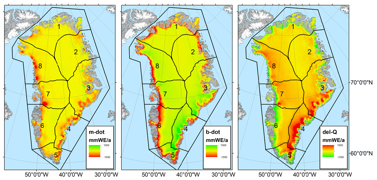
This new inversion mass balance product, which we are calling “HIGA” (Hybrid glacier Inventory, Gravimetry and Altimetry), suggests that between 2003 to 2009 Greenland lost 292 ± 78 Gt/yr of ice and the Canadian Arctic lost  42 ± 11 Gt/yr of ice. While the majority of Greenland’s ice loss was associated with the ice sheet proper (212 ± 67 Gt/yr), peripheral glaciers and ice caps, which comprise < 5 % of Greenland’s ice-covered area, produced ~ 15 % of Greenland mass loss (38 ± 11 Gt/yr). A good reminder that ice loss from “Greenland” is not synonymous with ice loss from the “Greenland ice sheet”. Differencing our tri-constrained mass balance product from a simulated surface mass balance field allowed us to assess the ice dynamic component of mass balance (technically termed the “horizontal divergence of ice flux”). This residual ice dynamic field infers flux divergence (or submergent ice flow) in the ice sheet accumulation area and at tidewater margins, and flux convergence (or emergent ice flow) in land-terminating ablation areas. This is consistent with continuum mechanics theory, and really highlights the difference in ice dynamics between the ice sheet’s east and west margins.

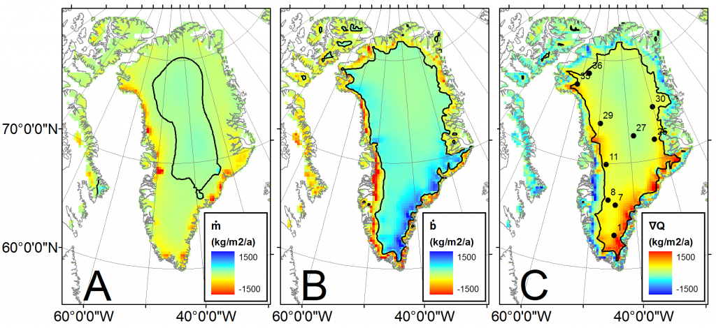
Figure 3 – Spatially partitioning the glacier continuity equation in surface and ice dynamic components. A: Transient glacier and ice sheet mass balance. B: Simulated surface mass balance. C: Residual ice dynamic (or horizontal divergence of ice flux) term. The ∇Q color scale is reversed to maintain blue shading for mass gain and red shading for mass loss in all subplots. Color scales saturate at minimum and maximum values. Black contours denote zero.

As with some scientific publications, this one has a bit of a backstory. In this case, we submitted a preliminary version of the study to The Cryosphere in December 2013. After undergoing three rounds of review at The Cryosphere, the first one of which is archived in perpetuity here, it was rejected, primarily for insufficient treatment of the uncertainty associated with firn compaction. Coincidentally, on the same day I received The Cryosphere rejection letter, I received a letter from the European Space Agency (ESA) granting funding for a follow-up study. A mixed day on email indeed! After substantial retooling, including a discussion section dedicated to firn compaction and the most conservative error bounds conceivable, we were happy to see this GRACE-ICESat study funded by NASA and the Danish Council for Independent Research appear in Remote Sensing of Environment. The editors at both journals, however, were very helpful in moving us forward. Our ESA-funded GRACE-CryoSat product development is now ongoing, but a sneak peek is below.

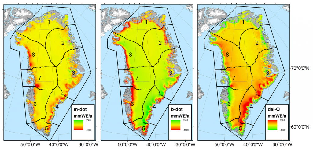
Figure 4 – Same as Figure 3, except using a 5 km resolution GRACE-CryoSat inversion product instead of a 26 km resolution GRACE-ICESat inversion product. Colorbars are different in shading, but identical in magnitude.

Reference

¹W. Colgan, W. Abdalati, M. Citterio, B. Csatho, X. Fettweis, S. Luthcke, G. Moholdt, S. Simonsen, M. Stober. 2015. Hybrid glacier Inventory, Gravimetry and Altimetry (HIGA) mass balance product for Greenland and the Canadian Arctic. Remote Sensing of Environment. 168: 24-39.

Our new #Greenland mass balance product assimilates satellite gravimetry and altimetry data: http://t.co/4FucwYzUGA pic.twitter.com/Kbekmq6uUU

— William Colgan (@GlacierBytes) July 7, 2015

We have a new study coming out in Earth and Planetary Science Letters that looks into the mass loss of the Greenland ice sheet (Andersen et al., 2015). We used the “input-output” approach, whereby an estimated iceberg production rate is differenced from an estimated snow accumulation rate. The input-output approach we used was slightly different from previous studies (such as Rignot et al., 2008 or Enderlin et al., 2014) because the ice sheet perimeter across which we observed ice flow (or the “flux gate”) was relatively far inland. That meant we had to make a different assumption about the vertical velocity profile at the flux gate, as well as account for changes in ice volume between the flux gate and the tidewater glacier grounding lines. We also used a new combination of satellite-derived ice surface velocity product, airborne radar-derived ice thickness observations, and surface mass balance simulations. Despite all this, our mass loss estimate agrees pretty well with previous studies!

The numbers are pretty striking: We estimate that between 2007 and 2011 the Greenland ice sheet alone, not counting all the peripheral glaciers in Greenland, lost 262 Gt of ice per year. That works out to about 8300 tonnes per second! That means the Greenland ice sheet probably weighs 250,000 tonnes less than when you started reading this blog post. No wonder we can measure its mass loss by gravitational anomalies! The ice sheet is currently losing mass via both surface runoff (the difference between accumulation and melt) and ice dynamics (the production of icebergs). We estimate that runoff comprised about 61 % of the ice sheet’s mass loss, or about 5000 tonnes per second, with iceberg production comprising the remaining 3300 tonnes per second of mass loss. Some big numbers that confirm the Greenland ice sheet is presently raising global mean sea level by about 0.73 mm per year.

Enderlin, E., I. Howat, S. Jeong, M. Noh, J. van Angelen & M. van den Broeke. 2014. An improved mass budget for the Greenland ice sheet. Geophysical Research Letters. 41: doi:10.1002/2013GL059010.

Rignot, E., J. Box, E. Burgess & E. Hanna. 2008. Mass balance of the Greenland ice sheet from 1958 to 2007. Geophysical Research Letters. 35: doi:10.1029/2008GL035417.

Andersen, M., L. Stenseng, H. Skourup, W. Colgan, S. Khan, S. Kristensen, S. Andersen, J. Box, A. Ahlstrøm, X. Fettweis & R. Forsberg. 2015. Basin-scale partitioning of Greenland ice sheet mass balance components (2007–2011). Earth and Planetary Science Letters. 409: 89–95. doi:10.1016/j.epsl.2014.10.015.

Diagram showing differences in methodology between our study (TOP) and previous studies (BOTTOM) in converted estimated ice flux (F) into estimated iceberg production (D). We adopt a higher elevation “flux gate”, which necessitates accounting for downstream changes in ice volume (∆S), as well as making a different assumption about the vertical velocity profile at the flux gate. We also use different velocity and ice thickness observations, and a different surface mass balance (SMB) model (from Andersen et al., 2015).