BLOG

We have a new article in the current issue of Geophysical Research Letters that looks at the influence of Greenland’s peripheral glaciers on vertical bedrock motion. Greenland’s bedrock is currently uplifting, due to both slow mantle-deformation processes associated with ice loss at the end of the Last Glacial Period, and fast elastic processes associated with ice loss today. The vertical bedrock uplift being measured in Greenland today ranges from a couple millimeters to a couple centimeters across the country. Understanding the magnitude and spatial distribution of this uplift helps us understand not only recent ice loss, but also properties of the Earth’s mantle beneath Greenland.

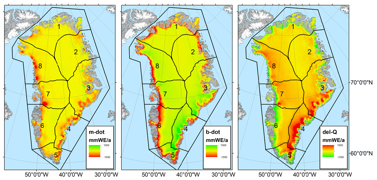
When folks create maps of Greenland’s present-day uplift rate, they typically use a model of changing ice-sheet geometry through time, to incorporate the effect of changing ice load on the Earth’s crust. This captures the main signal, but it ignores the cumulative effect of Greenland’s thousands of peripheral glaciers. These glaciers, which surround the ice sheet, also effect vertical bedrock motion. In this study, we also incorporate the effect of changing peripheral glacier geometry through time into uplift rates calculated at all the GNET bedrock motion sites around Greenland. In the figure above, you can see the vertical land motion budget of MSVG (Mestersvig) GNET station, which calculates post-Last Glacial Period glacioisostatic adjustment (GIA) as the residual of present-day elastic rebound.

We find that peripheral glaciers can have a disproportionately large impact on the elastic rebound of GNET sites, especially when they are located relatively far from the ice sheet. In some regions, especially in Greenland’s north and northeast, peripheral glaciers can contribute to over 20% of the total elastic response of regional GNET sites. Simply put, mapping Greenland’s present-day uplift rate with models that only incorporate the ice sheet, and not peripheral glaciers, can really underestimate the elastic rebound associated with present-day ice loss. Under estimating present-day elastic rebound can result in subsequently over estimating the post-Last Glacial Period glacioisostatic adjustment that is used to infer mantle properties.

So, perhaps the main message of this study is that although Greenland’s peripheral glaciers are quite small in comparison to the ice sheet, their recent collective ice loss can influence our understanding of Greenland’s vertical land motion in a disproportionately large way!

Open-Access Study: Berg, D., Barletta, V. R., Hassan, J., Lippert, E. Y. H., Colgan, W., Bevis, M., et al. (2024). Vertical land motion due to present-day ice loss from Greenland’s and Canada’s peripheral glaciers. Geophysical Research Letters, 51, e2023GL104851. https://doi.org/10.1029/2023GL104851

We have a new open-access study linking bedrock uplift and iceberg discharge at three major Greenland outlet glaciers in the last issue of Geophysical Research Letters. We look at recent changes in observed uplift rates and ice discharges at Jakobshavn, Kangerlussuaq and Helheim Glaciers. The idea of the study was to explore what we thought was a rather straightforward relation between uplift and discharge – uplift rates are relatively high when discharge rates are relatively high (and vice versa) – and see if there as any predictive power in this relation.  

The uplift rates are observed at GNet GPS stations and the ice discharges are observed by satellite-derived ice velocity combined with knowledge of ice thickness. When we analyzed these records, we found that the uplift-discharge relation is indeed very statistically strong, but – rather counterintuitively – at two of the glaciers it was bedrock uplift that serves as a good predictor for ice discharge. Simply put, rather than changes in bedrock uplift lagging changes in ice discharge, we instead found that changes in ice discharge lag changes in bedrock uplift. Clearly, surface mass balance is the primary and instantaneous driver of elastic bedrock uplift; bedrock uplift increases immediately after a big melt and runoff event. We are effectively showing that the associated ice discharge response is lagged.

At Jakobshavn Glacier, changes in ice discharge appear to lag changes in bedrock uplift by almost one year (0.87 years). Simply put, if there is a big melt and uplift event in August, the ice discharge response will peak the following June. If we trust this relation, recent uplift observations at Jakobshavn Glacier suggest that ice discharge will return to pre-2018 levels by the end of 2021. This would mark a clear end to a three-year period of relatively low ice discharge and ice-sheet thickening in the lower reaches of the ice stream over the 2016-2018 melt seasons. At Helheim Glacier, by contrast, there was no significant lead or lag; changes in uplift rate seem completely coincident with changes in ice discharge. Simply put, peak uplift and ice dischrage tends to be simultaneous.

You can speculate that this uplift-discharge relation changes from glacier to glacier around Greenland due on local differences in bedrock geology and glacier dynamics or hydrology. Reflecting, for example, the elastic modulus of the bedrock or the reservoir time of englacial hydrology of each glacier. The sensitivity of this relation – meaning how many mm/yr uplift per Gt/yr mass loss – also varies from GPS station to GPS station based on the local ice configuration and distance of the GPS station to the center of ice loss. These relations are therefore only valid over local scales.

Overall, however, it does seem possible to use the GNet stations to develop local relations between bedrock uplift and ice discharge on a glacier-by-glacier basis all the way around Greenland. This would be very helpful for using GPS stations to reconstruct detailed records of local ice loss prior to the 2016 onset of weekly satellite monitoring of ice discharge. Exploring this uplift-discharge relation at more GNet stations may also help us understand exactly why sub-annual changes in ice discharge appear to be lagging changes in vertical bedrock motion at some glaciers. Any new clues about processes that regulate Greenland’s ice discharge into the ocean are always valuable!

Hansen, K., Truffer, M., Aschwanden, A., Mankoff, K., Bevis, M., Humbert, A., van den Broeke, M., Noel, B., Bjørk, A., Colgan, W., Kjær, K., Adhikari, S., Barletta, V., and S. Khan. (2021). Estimating ice discharge at Greenland’s three largest outlet glaciers using local bedrock uplift. Geophysical Research Letters, 48, e2021GL094252. https://doi.org/10.1029/2021GL094252

We have just completed a study that inventories Arctic land ice loss since 1971. It is available open-access in the current issue of Environmental Research Letters¹. While we scientists have a pretty good idea of the health — or mass balance — of glaciers and ice sheets — or land ice — since the advent of satellite altimetry in the early 1990s, there is a need for better understanding of land ice health during the pre-satellite era. Our new study estimates the annual ice loss from all glacierized regions north of 55°N between 1971 and 2017.

We use in situ data – mass balance measurements from a handful of continuously monitored glaciers – as indicators for the health of land ice in seven Arctic regions. These hard-fought in situ data are scarce, they are only measured at between 20 and 44 Arctic glaciers every year. Extrapolating these data to entire regions is statistically challenging without additional information. Fortunately, independent estimates of regional mass balance are available from satellite gravimetry during the 2003 to 2015 period. This permits calibrating in situ and satellite-derived mass balance estimates during the satellite era. This makes our pre-satellite era estimates fairly robust.

During the 41 years assessed, we estimate that approximately 8,300 Gt of Arctic land ice was lost. It is difficult to contextualize this magnitude of ice loss. The flow of Niagara Falls – which is approximately 2400 m³ per second or about 75 km³ per year – is only equivalent to about half this volume (3500 km³) over the 1971-2017 period. The total Arctic land ice loss that we document represents 23 mm of sea-level rise since 1971. Greenland is by far the largest contributor (10.6 mm sea-level equivalent), followed by Alaska (5.7 mm sea-level equivalent) and then Arctic Canada (3.2 mm sea-level equivalent).

The UN Intergovernmental Panel on Climate Change (IPCC) now highlights two periods – the “recent past” (1986-2005) and “present day” (2005-2015) – as being of special interest in climate change studies. The Arctic land ice contribution to sea-level rise that we inventory increased from 0.4 to 1.1 mm sea-level equivalent between these periods. In terms of tonnes per second (5,000 to 14,000 t/s), both the magnitude – and the increase – are staggering.

Figure 1 – The cumulative sea-level rise contribution (in mm) from land ice in seven regions of the Arctic between 1971 and 2017. Analogous estimates from satellite gravimetry (GRACE) between 2003 and 2015 shown with open symbols.

The uncertainties associated with extrapolating sparse in situ data over large areas are undeniably large. But, the reality is that climate change was already gearing up as the global satellite observation network came online. So, in the absence of satellite data that can characterize the “pre-climate change” health of Arctic land ice, we need to leverage the extremely precious pre-satellite era observations that are available in creative ways. We hope that the ice loss estimates we present will be useful comparison targets for studies that estimate pre-satellite era mass balance in other ways.

The estimates of annual land ice mass balance — or health — in seven Arctic regions produced by this study are freely available for download here. This study was developed within the Arctic Monitoring and Assessment Program (AMAP) and International Arctic Science Committee (IASC) frameworks, as a direct contribution to the IPCC Special Report on the Ocean and Cryosphere in a Changing Climate (SROCC).

Figure 2 – Annual land ice mass balance — or health — in six Arctic regions between 1971 and 2017. Individual glacier mass balance records (blue lines) are combined into a regional composite (black line). Health is expressed both as a normalized score (left axis) and in gigatonnes per year (right axis). The numbers of glaciers comprising each composite is indicated in red text.

¹Box, J., W. Colgan, B. Wouters, D. Burgess, S. O’Neel, L. Thomson and S. Mernild. 2018. Global sea-level contribution from Arctic land ice: 1971 to 2017. Environmental Research Letters.

Our study assessing Arctic glacier loss since 1971 is out today.
I've written about *billions* of tonnes of ice loss before, but this is my first time writing about sea-level rise from *trillions* of tonnes. 🌊🙄
blog: https://t.co/GP880GMNpl
study: https://t.co/KSUXDTtBpS pic.twitter.com/Rz95RmIg1t

— William Colgan, Ph.D. (@GlacierBytes) December 21, 2018

We have a new review paper on glacier crevasses in the current issue of Reviews of Geophysics¹. We survey sixty years of crevasse studies, from field observations to numerical modeling to remote sensing of crevasses, and also provide a synthesis of ten distinct mechanisms via which crevasses influence glacier mass balance.

Two years ago, our team embarked on what was supposed to be a brief review of crevasse science to help interpret maps of Greenland crevasse extent that we are generating from laser altimetry data as part of a NASA project entitled “Assessing Greenland Crevasse Extent and Characteristics Using Historical ICESat and Airborne Laser Altimetry Data”. The final review ended up containing 250 references and being 43 typeset pages in length. Evidently we found the crevasse life cycle contained more nuances than we had initially assumed! Here are some of the highlights that have shifted our paradigm:

Field observations – Although crevasses are conventionally conceptualized to initiate at the surface and propagate downwards, we were surprised to find compelling evidence that at least some crevasses initiate at several metres depth, before propagating upwards to appear at the glacier surface. For example, observations that new crevasses can intersect relict crevasses at angles as low as 5 ° indicates that the stresses governing fracture are below the depth of relict crevasses (as relict crevasses do not serve as stress foci). This has implications for interpreting “buried” crevasses as relict or active.

Figure 1 – Measured principal strain rates and crevasse locations observed circa 1995 at Worthington Glacier, USA². The cross-cutting of relict crevasses by active crevasses indicates relative crevasse chronologies can exist at a single point on a glacier.

Numerical modeling – While crevasses have conventionally been assumed to form perpendicular to principal extending stresses on glaciers, we were intrigued to find strong model evidence that non-trivial crevasse curvature and rotation can result when there is substantial shearing (Mode III fracture) acting in addition to the more the common opening (Mode I fracture). The role of such mixed-mode fracture in shaping crevasse geometry has implications for interpreting curved / rotated crevasses as either deformed following opening or in equilibrium with local shear.

Figure 2 – Schematic illustrating the three modes of fracture: Mode I (opening), Mode II (sliding), and Mode III (tearing).

Remote Sensing – Remote sensing technologies for crevasse detection exhibited remarkable growth over the past 60 years. Real-time crevasse detection for traverse vehicles advanced from Cold War era rudimentary push-broom “dishpans”, which measured bulk electric current density of surrounding ice, to modern fully autonomous rovers capable of executing ground penetrating radar grids. In terms of satellite imagery, crevasses went from being manually delineated in the coarse resolution visible imagery that became available in the 1970s to now being automatically detected by feature tracking algorithms in higher resolution visible and synthetic aperture radar imagery.

Figure 3 – Left: Cold War era “dishpan” detection system that inferred crevasses from changes in bulk electric current density³. Right: An autonomous ground-penetrating radar unit (Yeti) being used to map near-surface buried crevasses at White Island, Antarctica. (Photo: Jim Lever)

Mass Balance Implications – While many studies have described individual mechanisms by which crevasses can influence glacier mass balance, we wanted to provide an overview of all the possible mechanisms, and we were fortunate enough to have a graphic artist help us do it in a single schematic. The mass balance implications of crevasses contain several counter-intuitive nuances. For example, crevasses can enhance basal sliding in the accumulation area and suppress basal sliding in the ablation area. Given their myriad mass balance implications, however, crevasses may serve as both indicators and agents of changing glacier form and flow.

Figure 4 – Schematic overview of the various processes through which crevassed surfaces influence glacier mass balance relative to non-crevassed surfaces: (1) increased solar energy collection and enhanced surface ablation, (2) increased turbulent heat fluxes and enhanced surface ablation, (3) decreased buried crevasse air temperatures and suppressed ice deformation, (4) increased bulk glacier porosity and enhanced ablation area water retention, (5) increased supraglacial lake drainage and suppressed accumulation area water retention, (6) increased supraglacial lake drainage and enhanced ice deformation, (7) attenuated transmission of hydrologic variability (relative to moulins) and suppressed basal sliding velocities, (8) increased cryo-hydrologic warming of ice temperatures and enhanced ice deformation, (9) increased water content / hydraulic weakening and enhanced ice deformation, and (10) iceberg calving.

¹Colgan, W., H. Rajaram, W. Abdalati, C. McCutchan, R. Mottram, M. S. Moussavi and S. Grigsby. 2016. Glacier crevasses: Observations, models, and mass balance implications. Reviews of Geophysics. 54: doi:10.1002/
2015RG000504.

²Harper, J., N. Humphrey and W. Pfeffer. 1998. Crevasse patterns and the strain-rate tensor: A high-resolution comparison. Journal of Glaciology. 44: 68–76.

³Mellor, M. 1963. Oversnow Transport. Cold Regions Science and Engineering. Monograph III-A4. 104 pages.

Intro to our review paper on #glacier crevasses. https://t.co/7au4CCjaIf
(Published Feb 29 in Rev. Geophys.) pic.twitter.com/cXSFacETMT

— William Colgan (@GlacierBytes) March 1, 2016

Jamieson and colleagues published a very neat investigation of the applied glaciology challenges at Kumtor Mine, Kyrgyzstan, this week in the AGU Journal of Geophysical Research: Earth Surface (open access here). The recovery of subglacial gold deposits at Kumtor Mine has necessitated the excavation of an open ice pit into the Lysii and Davidov Glaciers. In addition to excavating glacier overburden, a major geotechnical challenge at Kumtor Mine has been managing the flow of both glaciers. In their study, Jamieson et al. (2015) use a comprehensive set of high resolution satellite images to document recent artificial surges induced in both these glaciers in response to mining activities. Photos released by Radio Free Europe in 2013 suggest that these artificial surges quite adversely impacted mining operations (Figure 1).

Figure 1 – Infrastructure damage resulting from what is now a confirmed glacier advance at the Kumtor Mine in Kyrgyzstan (originally discussed in this earlier post)

The dumping of waste rock on both glaciers, in which waste rock piles reached up to 180 m thick, substantially increased the driving stress of the ice beneath. Given that ice deformation is related to driving stress to an exponent of three, and potentially higher exponents at higher driving stresses, this resulted in a significant increase in ice velocity. Jamieson et al. (2015) estimate that surface velocities of the Davidov Glacier increased from a few meters per year to several hundred meters per year within a decade. During this time, the Lysii and Davidov Glaciers advanced by 1.2 and 3.2 km, respectively, with Davidov Glacier terminus advance reaching 350 meters per year in c. 2012 (Figure “7”).

This study is probably the most textbook-comprehensive documentation of a human-induced artificial glacier surge to date, and will provide a great resource for my students to debate the sometimes fine line between geotechnical misstep and natural hazard!

Reference

(Jamieson, S., M. Ewertowski and D. Evans. 2015. Rapid advance of two mountain glaciers in response to mine-related debris loading. Journal of Geophysical Research: Earth Surface. 120: doi:10.1002/2015JF003504.

Quick blog on new study of human-induced 3.2 km #glacier surge at #Kumtor mine: http://t.co/mTYVeQDzcb pic.twitter.com/ONMkQETlRm

— William Colgan (@GlacierBytes) July 27, 2015

We have a new study in this month’s Remote Sensing of Environment, which examines satellite-derived glacier mass balance in Greenland and the Canadian Arctic¹. Satellites are generally used to assess glacier mass balance through changes in volume (via satellite altimetry) or changes in mass (via satellite gravimetry). While satellite altimetry observes volume changes at relatively high spatial resolution, it necessitates the forward modeling of firn processes to convert volume changes into mass changes. Conversely, the cryosphere-attributed mass changes observed by satellite gravimetry, while very accurate in absolute terms, have relatively low spatial resolution. In this study, we sought to combine the complementary strengths of both approaches. Using an iterative inversion process that was essentially sequential guess-and-check with a supercomputer, we refined gravimetry-derived observations of cryosphere-attributed mass changes to the relatively high spatial resolution of altimetry-derived volume changes. This gave us a 26 km spatial resolution mass balance field across Greenland and the Canadian Arctic that was simultaneously consistent with: (1) glacier and ice-sheet extent derived from optical imagery, (2) cryospheric-attributed mass trends derived from gravimetry, and (3) ice surface elevation changes derived from altimetry. We have made digital versions of this product available in the supplementary material associated with the publication.

Figure 1 – Observational data inputs to our inversion algorithm. A: Cryosphere-attributed mass changes observed by gravimetry. B: Land ice extent observed by optical imagery. C: Ice surface elevation changes observed by altimetry.

To make sure our inferred mass balance field was reasonable, we evaluated it against all in situ point mass balance observations we could find. Statistically, the validation was great, yielding an RMSE of 15 cm/a between the inversion product and in situ measurements. Practically, however, this apparent agreement largely stems from the fact that we could only find forty in situ point mass balance observations against which to compare. Evaluating our area-aggregated sector-scale mass balance estimates against all previously published sector-scale estimates provides a more meaningful validation. This suggests the magnitude and spatial distribution of inferred mass balance is reasonable, but highlights that the community needs more in situ point observations of mass balance, especially from peripheral glaciers and regions of high dynamic drawdown in Greenland. (For the glaciology hardcores I will note that “mass balance” is distinct from “surface mass balance”, in that the former measurement also includes the ice dynamic portion of mass change.)

Figure 2 – A comparison of similar sector scale mass balance estimates and associated uncertainties across Greenland and the Canadian Arctic. Dashed lines denote estimates that pertain to the Greenland ice sheet proper (i.e. exclusive of peripheral glaciers). Jacob et al. (2012) estimates pertain to Canada, while Sasgen et al. (2012) estimates pertain to Greenland.

This new inversion mass balance product, which we are calling “HIGA” (Hybrid glacier Inventory, Gravimetry and Altimetry), suggests that between 2003 to 2009 Greenland lost 292 ± 78 Gt/yr of ice and the Canadian Arctic lost  42 ± 11 Gt/yr of ice. While the majority of Greenland’s ice loss was associated with the ice sheet proper (212 ± 67 Gt/yr), peripheral glaciers and ice caps, which comprise < 5 % of Greenland’s ice-covered area, produced ~ 15 % of Greenland mass loss (38 ± 11 Gt/yr). A good reminder that ice loss from “Greenland” is not synonymous with ice loss from the “Greenland ice sheet”. Differencing our tri-constrained mass balance product from a simulated surface mass balance field allowed us to assess the ice dynamic component of mass balance (technically termed the “horizontal divergence of ice flux”). This residual ice dynamic field infers flux divergence (or submergent ice flow) in the ice sheet accumulation area and at tidewater margins, and flux convergence (or emergent ice flow) in land-terminating ablation areas. This is consistent with continuum mechanics theory, and really highlights the difference in ice dynamics between the ice sheet’s east and west margins.

Figure 3 – Spatially partitioning the glacier continuity equation in surface and ice dynamic components. A: Transient glacier and ice sheet mass balance. B: Simulated surface mass balance. C: Residual ice dynamic (or horizontal divergence of ice flux) term. The ∇Q color scale is reversed to maintain blue shading for mass gain and red shading for mass loss in all subplots. Color scales saturate at minimum and maximum values. Black contours denote zero.

As with some scientific publications, this one has a bit of a backstory. In this case, we submitted a preliminary version of the study to The Cryosphere in December 2013. After undergoing three rounds of review at The Cryosphere, the first one of which is archived in perpetuity here, it was rejected, primarily for insufficient treatment of the uncertainty associated with firn compaction. Coincidentally, on the same day I received The Cryosphere rejection letter, I received a letter from the European Space Agency (ESA) granting funding for a follow-up study. A mixed day on email indeed! After substantial retooling, including a discussion section dedicated to firn compaction and the most conservative error bounds conceivable, we were happy to see this GRACE-ICESat study funded by NASA and the Danish Council for Independent Research appear in Remote Sensing of Environment. The editors at both journals, however, were very helpful in moving us forward. Our ESA-funded GRACE-CryoSat product development is now ongoing, but a sneak peek is below.

Figure 4 – Same as Figure 3, except using a 5 km resolution GRACE-CryoSat inversion product instead of a 26 km resolution GRACE-ICESat inversion product. Colorbars are different in shading, but identical in magnitude.

Reference

¹W. Colgan, W. Abdalati, M. Citterio, B. Csatho, X. Fettweis, S. Luthcke, G. Moholdt, S. Simonsen, M. Stober. 2015. Hybrid glacier Inventory, Gravimetry and Altimetry (HIGA) mass balance product for Greenland and the Canadian Arctic. Remote Sensing of Environment. 168: 24-39.

Our new #Greenland mass balance product assimilates satellite gravimetry and altimetry data: http://t.co/4FucwYzUGA pic.twitter.com/Kbekmq6uUU

— William Colgan (@GlacierBytes) July 7, 2015